Factors Are Not Commodities

“A MAN WITH TWO WATCHES IS NEVER SURE [WHAT TIME IT IS].” 

SEGAL’S LAW (EXCERPT) 

A price-war is underway in the ETF industry, which assumes that factor-based products are commodities. We demonstrate that strategies built with different factor signals are not substitutes for one another. 

• Factor definitions matter. The way you adjust for a simple thing like price-to-earnings (P/E) can lead to significant differences in returns.
• Complexity does not equal effectiveness. Overfitted models lead to poorer factor returns.

The narrative put forth by smart beta products is that factors are becoming an investment commodity. Factors are not commodities—rather, they are unique expressions of investment themes. The uniqueness of one Value strategy from another can lead to very different results, and there are many places that factor- based portfolios can diverge. So the challenge for asset allocators is identifying exactly where and how these factor strategies differ one from another, even when they all claim to use the same themes of Value, Momentum, and Quality.

Over the past couple of years, several multi-factor funds that combine Value, Momentum, and Quality were launched. As these products compete to garner assets, price competition has started among rivals. In December, Blackrock cut fees to its smart beta ETFs¹ to compete with Goldman Sachs, which has staked out a cost leadership position in that market space. Michael Porter, the expert in competitive strategy, wrote in 1980 that there are three generic strategies that can be applied to any business for identifying a competitive advantage: cost leadership, differentiation, or focus.² Cost leadership can be an effective strategy, but the key to any price war is for the products to be near-perfect substitutes for one another, just like commodities. This paper focuses on how quantitative asset managers can have significant differences—in factor definitions, in combining factors into investment themes, and in portfolio construction techniques—leading to a wide range of investment experiences in multi-factor investment products. 

Factor Definition Discrepancies 

Value investing through ratios seems to be very straightforward. Price-to-earnings ratios are widely accepted as a common metric for gauging the relative cheapness of one stock versus another. A study by Asquith, Mikhail, and Au titled “Information Content of Equity Analyst Reports” found that 99 percent of equity analyst reports use earnings multiples in analyzing a company. P/E ratio is used widely because it’s straightforward and makes intuitive sense: as an equity owner you are entitled to the residual earnings of the company after expenses, interest, and taxes. Simply put, P/E tells you how much you’re paying for every dollar of earnings. 

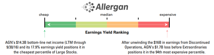
Procuring a P/E ratio is easy as opening up a web browser and typing in a search. But if you’ve ever compared P/E ratios from multiple sources, you can get a variety different numbers for the same company. For example, take a look at Allergan (NYSE: AGN). As of January 12, 2017, Yahoo! Finance had AGN with a P/E of 6.06. But Google Finance had 15.84. If you have access to a Bloomberg terminal, Bloomberg had it as a P/E of 734. On the other hand, FactSet has no P/E ratio. It’s like being stuck in Arthur Bloch's Segal’s Law: “A man with a watch knows what time it is. A man with two watches is never sure.”³

These discrepancies happen because there are many different ways to put together a P/E ratio. One way could use earnings per share divided by the price of the stock. If so, should “basic” or “diluted” EPS be used? There’s a difference if you switch to the LTM Net Income divided by the total market cap of the company, as shares can change over a given quarter. But the reason for Allergan’s different ratios is that some financial information providers use bottom-line earnings while others take Income before Extraordinaries and Discontinued Operations. In August 2016, Teva (NYSE: TEVA) acquired Allergan’s generics business “Actavis Generics” for $33.4 billion in cash plus 100 million Teva shares, generating earnings of $16 billion from Discontinued Operations. After unwinding this, the company actually lost $1.7 billion in 3Q16—hence no P/E ratio. Depending on whether or not an adjustment is made on this, Allergan would be positioned either as a cheapest percentile stock based on its Earnings Yield (inverse of the P/E ratio) or all the way down into the 94th percentile. 

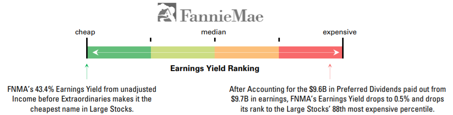
Accounting adjustments for Extraordinaries and Discontinued Operations aren’t the only item affecting an earnings ratio. When considering earnings, you really want to measure the available economic surplus that flows to the holder of the common equity. If preferred stock exists, it supersedes the claims of common shareholders. Fannie Mae (OTC: FNMA) is a great example of how preferred dividends can absorb earnings from common shareholders. During the 2008 crisis, Fannie Mae issued a senior tranche of preferred stock that is owned by the U.S. Treasury, and is paying a $9.7 billion dividend of the company’s $9.8 billion in earnings. There is a junior preferred tranche held by investors like Pershing Square and Fairholme Funds—they are currently not receiving dividends and are submitting legal challenges to receive some portion of the earnings. This leaves common shareholders behind a long line of investors with prioritized claims on earnings. But some methodologies’ adjusted earnings take preferred dividends after earnings, while others do not, creating a difference in having a P/E of 2.3 (an Earnings Yield of 43 percent) or a P/E of 185 (Earnings Yield of 0.5 percent). 

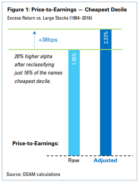
These comments are not about the cheapness of Allergan or Fannie Mae. Instead, it shows the importance of your definition of “earnings” and the adjustments you apply. If these considerations sound like fundamental investing, it’s because they are. Fundamental analysts consider these adjustments in the analysis of a company. Factor investors work through the same accounting issues as fundamental investors, with the additional burden of trying to make systematic adjustments to create a stronger metric that acknowledges the accounting differences across thousands of companies. Investing results can vary greatly based on these adjustments. In the U.S. Large Stocks Universe,⁴ there is a +38bps improvement on the highest decile of Earnings Yield if you adjust for Discontinued Items, Extraordinaries, and Preferred Dividends (see Figure 1 below). To set some comparative scale using eVestment’s peer analysis, the difference between a median manager and a top quartile manager is +60bps a year. 

Adjustments to Value signals are not limited to price-to-earnings. Book Value can be adjusted for the accounting of Goodwill and Intangibles. Dividend yield can be calculated using the dividends paid over the trailing 12-months, or annualizing the most recent payment. In 2004, Microsoft paid out $32 billion of its $50 billion in cash in a one-time $3 per share dividend when the stock was trading at around $29. Knowing that future investors won’t receive similar dividend streams, should that dividend get included in calculating yield? 

Differences in signal construction are not limited to Value factors. Momentum investors know that there are actually three phenomena observed in past price movement: short-term reversals in the first month, medium-term momentum over the next 12 months, and long-term reversals over a 3- to 5-year period. Put two Momentum investors in a room and they will disagree over whether or not to delay the momentum signal by one month to avoid reversals (i.e., the 12-months minus one month). Quality investors argue the use of non-current balance sheet items, or the loss of effectiveness in investing on changes in analyst estimates. Volatility can be measured using raw volatility, beta, or idiosyncratic volatility, to name just a few methods. 

Factors are constructed as unique expressions of an investment idea and are not the same for everyone. Small differences can have large impact on which stocks make it into the portfolios. These effects are even more significant when using an optimizer (potentially maximizing errors) or when concentrating portfolios (thereby giving more weight to individual names). 

There is skill in constructing factors—far from simply grabbing a P/E ratio from a Bloomberg data feed. 

Alpha Signals 

Quantitative managers tend to combine individual factors together into themes like Value, Momentum, and Quality. But there are several ways that managers can combine factors into models for stock selection. And models can get very complicated. In the process of manager selection, allocators have the difficult task of gauging the effectiveness of these models. The common mistake is assuming complexity equals effectiveness. 

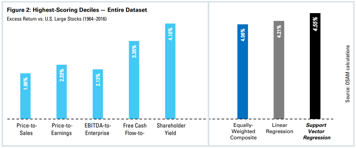
To demonstrate how complexity can degrade performance, let’s take five factors in the Large Stocks space and aggregate them into a Value theme: Price/Sales, Price/Earnings, EBITDA/EV, Free Cash Flow/Enterprise Value, and Shareholder Yield (a combination of dividend and buyback yield). 

The most straightforward is an equally-weighted model: give every factor the same weight. This combination of the five factors generates an annual excess return of 4.06 percent in the top decile. An ordinary linear regression increases the weighting of Free Cash Flow-to-Enterprise Value, and lowers the weighting on Price-to-Earnings because it was less effective over that time frame. This increases the apparent effectiveness by +15bps (annualized)—not a lot, but remember this is Large Cap where edge is harder to generate. Other linear regressions, like ridge or lasso, might be used for parameter shrinkage or variable selection and try to enhance these results. 

Moving up the complexity scale, non-linear or machine learning models like Neural Networks, Support Vector Machines, or Decision Trees can be used to build the investment signal. There has been a lot of news around Big Data and the increased usage of machine learning algorithms to help predict outcomes. For the example in Figure 2, we’ve built an approach using a Support Vector Regression, a common non-linear machine-learning technique. At first glance, the Support Vector Regression looks very effective, increasing the outperformance of selecting stocks on Value to 4.55 percent, almost a half of a percent annualized return over the equally weighted model. 

The appeal of a machine-learning approach is strong. Intuitively, the complex process should do better than the simple, and the first pass results look promising. But this apparent edge does not hold up on examination. 

This apparent edge is from overfitting a model. Quantitative managers might have different ways of constructing factors, but we are all working with data that does not change as we research ideas: quarterly financial and pricing data back to 1963. As we build models, we can torture that data to create the illusion of increased effectiveness. The linear regression and support vector machines are creating weightings out of the same data used to generate the results, which will always look better. 

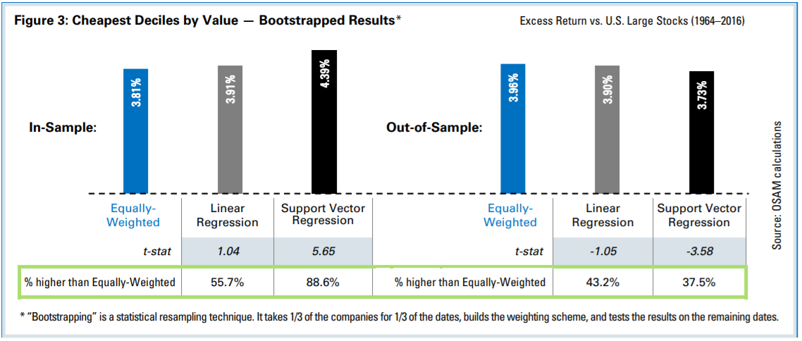
The statistical method to help guard against overfitting is bootstrapping. The process creates in-sample and out-of-sample tests by taking random subsamples of the dates, as well as subsets of the companies included in the analysis. Regression weightings are generated on an in-sample dataset and tested on an out-of-sample dataset. The process is repeated a hundred times to see how well the weighting process holds up. 

In the bootstrapped results, you can see how the unfitted equally-weighted model maintains its effectiveness at about the same level. The in-sample data in Figure 3 looks just like the first analysis: the linear regression does slightly better and the Support Vector Regression (SVR) does significantly better. When applying the highly-fitted SVR to the out-of-sample data, the effectiveness inverts. Performance degrades at a statistically significant level once you implement on investments that weren’t part of your training data. 

This doesn’t mean that all weighted or machine learning models are broken, rather that complex model construction comes with the risk of overfitting to the data and can dilute the edge of factors. Overfitting is not intentional, but a by-product of having dedicated research resources that are constantly looking for ways to improve upon their process. When evaluating the factor landscape, understand the model used to construct the seemingly similar themes of Value, Momentum or Quality. Complexity in itself is not an edge for performance, and makes the process less transparent to investors creating a “black box” from the density of mathematics. Simple models are more intuitive and likely to hold up in the true out-of-sample dataset, the future.

Various factor products can generate several hundreds of basis points of difference in a single year are not commoditized and should not be chosen for investment in because of a few basis points in fees. Cost leadership is the key feature for generic market-capitalization weighted schemes, but product differentiation and focus in the context of fees should be the reasons for investing in multi-factor products. 

SUMMARY 

There is significant edge in how factor signals are constructed. The difficulty is creating transparency around this edge for investors. Complexity of stock selection and construction methodology decreases transparency, almost as much as active quantitative managers that create a "black box" around their stock ranking methodologies. This leaves investors at a disadvantage when trying to differentiate between quantitative products. This inability to differentiate is why price wars are starting between products that have strong differences in features and results. 

Investors need education on this differentiation so they’re not selecting only on the lowest fees. Sophisticated manager selection focuses on people, philosophy, and process, as well as performance. These things will still matter in understanding a factor portfolio, but now they need to add expertise on understanding factors and portfolio construction. Large institutional and investment consultant manager selection groups will have the difficulty of adding top-tier quantitative investment staff to help with this differentiation. Smaller groups and individual investors will have to advance their own understanding of how quantitative products are constructed. For all of these factor investors, it will help to build trusted partnerships with quantitative asset managers willing to share insights on the factor investing landscape. 

Footnotes:

¹ See https://www.bloomberg.com/news/articles/2016-12-19/Blackrock-Cuts-Fees-on-ETFs-as-Price-War-Moves-to-Smart-Beta

² Porter, Michael, Competitive Strategy, Free Press, New York (1980)

³ Bloch, Arthur, Murphy’s Law (2003) 

⁴ The universe of Large Stocks consists of all securities with inflation-adjusted market cap greater than the universe average. The stocks are equally-weighted and rebalanced periodically. 

General Legal Disclosures & Hypothetical and/or Backtested Results Disclaimer 

The material contained herein is intended as a general market commentary. Opinions expressed herein are solely those of O’Shaughnessy Asset Management, LLC and may differ from those of your broker or investment firm. 

Please remember that past performance may not be indicative of future results. Different types of investments involve varying degrees of risk, and there can be no assurance that the future performance of any specific investment, investment strategy, or product (including the investments and/or investment strategies recommended or undertaken by O’Shaughnessy Asset Management, LLC), or any non-investment related content, made reference to directly or indirectly in this piece will be profitable, equal any corresponding indicated historical performance level(s), be suitable for your portfolio or individual situation, or prove successful. Due to various factors, including changing market conditions and/or applicable laws, the content may no longer be reflective of current opinions or positions. Moreover, you should not assume that any discussion or information contained in this piece serves as the receipt of, or as a substitute for, personalized investment advice from O’Shaughnessy Asset Management, LLC. Any individual account performance information reflects the reinvestment of dividends (to the extent applicable), and is net of applicable transaction fees, O’Shaughnessy Asset Management, LLC’s investment management fee (if debited directly from the account), and any other related account expenses. Account information has been compiled solely by O’Shaughnessy Asset Management, LLC, has not been independently verified, and does not reflect the impact of taxes on non-qualified accounts. In preparing this report, O’Shaughnessy Asset Management, LLC has relied upon information provided by the account custodian. Please defer to formal tax documents received from the account custodian for cost basis and tax reporting purposes. Please remember to contact O’Shaughnessy Asset Management, LLC, in writing, if there are any changes in your personal/financial situation or investment objectives for the purpose of reviewing/evaluating/revising our previous recommendations and/or services, or if you want to impose, add, or modify any reasonable restrictions to our investment advisory services. Please Note: Unless you advise, in writing, to the contrary, we will assume that there are no restrictions on our services, other than to manage the account in accordance with your designated investment objective. Please Also Note: Please compare this statement with account statements received from the account custodian. The account custodian does not verify the accuracy of the advisory fee calculation. Please advise us if you have not been receiving monthly statements from the account custodian. Historical performance results for investment indices and/or categories have been provided for general comparison purposes only, and generally do not reflect the deduction of transaction and/or custodial charges, the deduction of an investment management fee, nor the impact of taxes, the incurrence of which would have the effect of decreasing historical performance results. It should not be assumed that your account holdings correspond directly to any comparative indices. To the extent that a reader has any questions regarding the applicability of any specific issue discussed above to his/her individual situation, he/she is encouraged to consult with the professional advisor of his/her choosing. O’Shaughnessy Asset Management, LLC is neither a law firm nor a certified public accounting firm and no portion of the newsletter content should be construed as legal or accounting advice. A copy of the O’Shaughnessy Asset Management, LLC’s current written disclosure statement discussing our advisory services and fees is available upon request. 

The risk-free rate used in the calculation of Sortino, Sharpe, and Treynor ratios is 5%, consistently applied across time. 

The universe of All Stocks consists of all securities in the Chicago Research in Security Prices (CRSP) dataset or S&P Compustat Database (or other, as noted) with inflation-adjusted market capitalization greater than $200 million as of most recent year-end. The universe of Large Stocks consists of all securities in the Chicago Research in Security Prices (CRSP) dataset or S&P Compustat Database (or other, as noted) with inflation-adjusted market capitalization greater than the universe average as of most recent year-end. The stocks are equally weighted and generally rebalanced annually. 

Hypothetical performance results shown on the preceding pages are backtested and do not represent the performance of any account managed by OSAM, but were achieved by means of the retroactive application of each of the previously referenced models, certain aspects of which may have been designed with the benefit of hindsight. 

The hypothetical backtested performance does not represent the results of actual trading using client assets nor decision-making during the period and does not and is not intended to indicate the past performance or future performance of any account or investment strategy managed by OSAM. If actual accounts had been managed throughout the period, ongoing research might have resulted in changes to the strategy which might have altered returns. The performance of any account or investment strategy managed by OSAM will differ from the hypothetical backtested performance results for each factor shown herein for a number of reasons, including without limitation the following: 

• Although OSAM may consider from time to time one or more of the factors noted herein in managing any account, it may not consider all or any of such factors. OSAM may (and will) from time to time consider factors in addition to those noted herein in managing any account. 
• OSAM may rebalance an account more frequently or less frequently than annually and at times other than presented herein. 
• OSAM may from time to time manage an account by using non-quantitative, subjective investment management methodologies in conjunction with the application of factors. 
• The hypothetical backtested performance results assume full investment, whereas an account managed by OSAM may have a positive cash position upon rebalance. Had the hypothetical backtested performance results included a positive cash position, the results would have been different and generally would have been lower.
• The hypothetical backtested performance results for each factor do not reflect any transaction costs of buying and selling securities, investment management fees (including without limitation management fees and performance fees), custody and other costs, or taxes – all of which would be incurred by an investor in any account managed by OSAM. If such costs and fees were reflected, the hypothetical backtested performance results would be lower. 
• The hypothetical performance does not reflect the reinvestment of dividends and distributions therefrom, interest, capital gains and withholding taxes.
• Accounts managed by OSAM are subject to additions and redemptions of assets under management, which may positively or negatively affect performance depending generally upon the timing of such events in relation to the market’s direction. 
• Simulated returns may be dependent on the market and economic conditions that existed during the period. Future market or economic conditions can adversely affect the returns.