O’Shaughnessy Quarterly Investor Letter Q3 2018

Dear Investor,

Basic factor investing is settled territory. Most investors have been bludgeoned with countless strategies that use factors like value, momentum, quality, or low volatility. As William Gibson observed in Pattern Recognition, “commodification will soon follow identification.” The primary factors were identified long ago and have been packaged and repackaged in just about every way imaginable.

I’d like to use this letter to describe the more interesting, next stage of factor investing: alpha within factors. This simple idea describes what we’ve pursued at OSAM over the years, and what we continue to pursue through our research agenda today. We will soon be sharing a broader and more formal paper on alpha within factors, but as a precursor I’ll use this letter to illustrate what we mean through an abbreviated example: an exploration of buybacks, capital allocation, and the buyback factor. My goal is not to showcase our entire research process (which has a lot more nuance), but instead to highlight the spirit of how we search for useful signals.

In accordance with our mantra of “learn, build, share, repeat” I will also use statistical learning methods¹ as part of this analysis to show how useful they can be. Methods like the clustering technique described below help detect complex correlation structures in data sets. The identification of patterns can lead to insight, understanding, new ideas, and model improvements.

Why We Care About Buybacks

As a broad category, the stocks of companies which have repurchased large percentages of shares have outperformed the market. But within the sample of high buyback firms, there has been a wide dispersion of outcomes. The question I explore is whether we can model this dispersion to find alpha within the buyback factor.

First, it is helpful to review how important buybacks have become. Consider a new metric we call “Peak Yield,” which is the total reduction in shares outstanding from a company’s peak historical shares. Peak yield tells us how large a total buyback program a company has completed through a given date in history (e.g. Apple has repurchased 25% of its shares since 2013).

Here is Northrup Grumman as a visual example, including two periods of share buybacks. Its shares are shown in red, “peak shares” (the maximum amount shares outstanding in a given company’s history) are tracked in green, and peak yield (cumulative total buyback percentage since the share peak) is shown in blue.

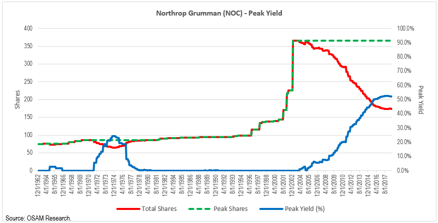
Since 2004 Northrup has steadily and aggressively repurchased 52% of its shares.

Here is the average peak yield of all stocks in the U.S., shown for both large and small stocks. The average large cap stock has repurchased 20% of its shares from the peak. This average includes all the companies which remain at their share peak (i.e. their peak yield = 0), which is roughly 20% of the large cap sample.

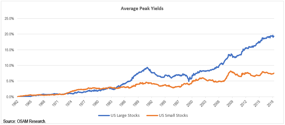
The average time since peak shares is more than 12 years, and the overall market’s buyback activity has been steady between 2% and 3% per year. Barring legislative action around buybacks, we expect companies to continue to use considerable amounts of cash to buy back shares.

Excess Returns

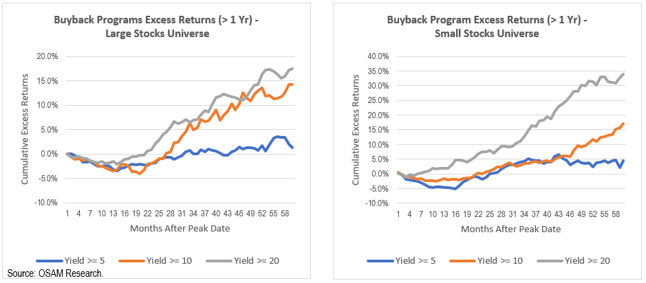
We are so interested in this factor because during (and after) these periods of significant share buybacks, these stocks have outperformed. Here is the average excess return of these stocks as they are repurchasing shares (where time zero is set at the peak share date for each company). We group companies by their buyback intensity. As you can see below where we group stocks into those that have repurchased more than 5% of share, more than 10% and more than 20%, the higher the cumulative buyback yield, the higher the excess return.

These are returns that happen alongside buybacks, but investors should only care about signals which are predictive of forward returns. Here are the results for a variety of simple buyback factors. The factors sort companies by looking back between 6 months and 10 years of trailing buyback activity.

Across the board, buying companies which have repurchased a large percent of shares in the past continue to outperform in the future. Companies in the lowest decile, which are issuing the most shares, perform poorly.

Even looking back ten years, or all the way to share peak, buyback factors have still delivered strong forward return spreads.

Capital Pies

Buybacks on their own seem to provide an interesting signal, but buybacks are just one of several potential uses of corporate cash. OSAM’s investing model places significant emphasis on capital allocation factors because we believe that with so much focus on the balance sheet and operating metrics, these factors are an underused and underappreciated source of differentiation.

Capital allocation factors also lend themselves to quantitative analysis because they can be summarized and measured in just a few major categories. We call these capital pies.

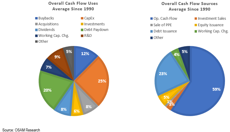
Spending Pie: cash can be spent on buybacks, dividends, debt paydown, capital expenditures, research & development, working capital, and acquisitionsⁱ.

Sourcing Pie: cash can be sourced from operating cash flow, debt issuance, equity issuance, sales of assets, and sale of investments.

Here are the sources and uses of cash for all large cap companies on average, based on data from the statement of cash flows. One important note: you’ll notice that while mergers and acquisitions are generally the largest use of capital, acquisition cash flow is a small slice here. That is because the capital for acquisitions comes from debt and equity issuance, and from existing cash. Only the use of existing cash (netted against any cash acquired) shows up here as a separate item.

What we are most interested in is whether different styles of capital allocation beyond buybacks lead to unique outcomes that we as investors can use in our process. One idea would be to use buyback intensity as a distinguishing factor for bucketing capital allocation styles. Doing so, we can create simple style groups:

1) Issuers (negative buyback yield)

2) Buybacks >=0

3) Buybacks >5% (high conviction)

4) Buybacks >10% (highest conviction)

This grouping does one thing well: it reflects the relative maturity of the companies within each group. Here is the average trailing five-year sales growth for each, showing that firms issuing shares tend to be growing much faster, and thus consuming more capital. Those with the highest buybacks are growing much slower.

By building the capital pies for each group, we begin to see how companies behave at different stages, starting with issuers on the left, and steadily higher buyback levels as we move right:

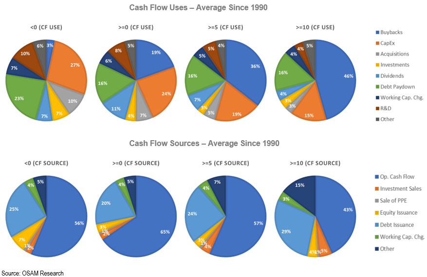
While there are some noticeable differences (issuers spend more on CAPEX and R&D, higher and higher buyback firms are more reliant on debt financing), the pies are very roughly similar. So perhaps our group isn’t ideal for producing further insight.

The Right Kind of Buyback

Each company is different, and no two capital allocation strategies will be exactly alike. But the entire quantitative research process is about finding common categories which perform in similar ways, so that we can then buy or avoid/sell short the categories. Rather than classify different styles of capital allocation manually (as we did above with levels of buyback activity), we can also use methods like clustering (k-means) to identify patterns for us. These patterns may point towards sources of alpha within factors.

For this exercise, we start with all companies with a positive buyback yield, and set the number of clusters to three, meaning the algorithm will create three capital allocation/sourcing “archetypes” and then assign every stock to one of three². To build the archetypes, the clustering algorithm needs data, so we feed it every slice of the capital pies for every company, on every date since 1990.

What I love about this method is that it classifies companies objectively, based on the most similar traits, and not based on our opinion of what the groupings should be. The resulting clusters are not delineated based on their buyback level as we tried above. Instead they are grouped based on the financing source and level of investment.

We will call these groups:

1) Internal financing, high investment

2) Mixed financing, mixed investment

3) Debt financing, low investment

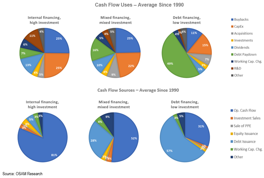
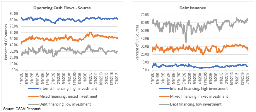
These relationships are much more distinct than we saw when we grouped companies by their buyback activity. Here is a time series of the percent of cash coming from operations vs. debt for the three clusters:

The internal financing companies spend the most (as a percent of total spending) on both CAPEX and R&D:

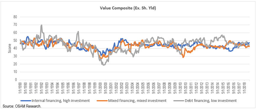
Here is the average relative valuation for each group (where the 50th percentile is the median valuation across all large stocks, and 1st percentile is cheapest stock). Companies buying back shares tend to be slightly cheaper than the market on average, and you can see that reflected here. But for the most part, the relative valuations of these groups are similar, despite very different capital sourcing and spending styles.

Now, here are the returns of each cluster since 1990, shown as excess returns vs. the overall group of positive buyback companies. The internally financed, high investment group outperformed the debt financing, low investment group by 3% per year, annually. That is a large number in a large cap universe, keeping in mind that most common factors usually applied in this space (value, momentum, etc.) are entirely absent here.

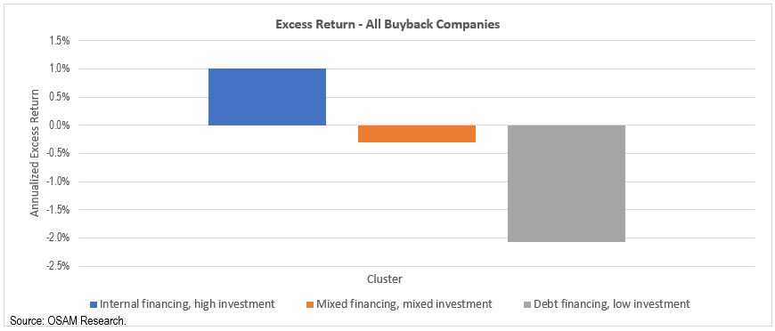
This tells us that financing source is likely a robust way to generate alpha within the buyback factorⁱⁱ.

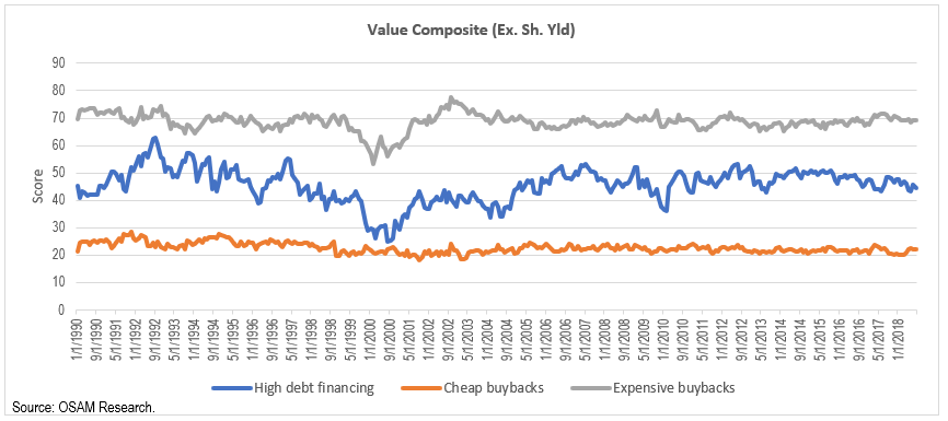
We return to our clustering algorithm, but add the valuation score shown above as a variable when building the clusters, so now we are grouping stocks based on their capital pies and their current valuation. We do so because intuitively, the price at which buybacks are happening should be critical. If a management team repurchases shares below intrinsic value, that is good decision for shareholders (and if they do so at a premium, it’s a bad decision). With valuation added, different clusters emerge.

1) High debt financing

2) Cheap buybacks

3) Expensive buybacks

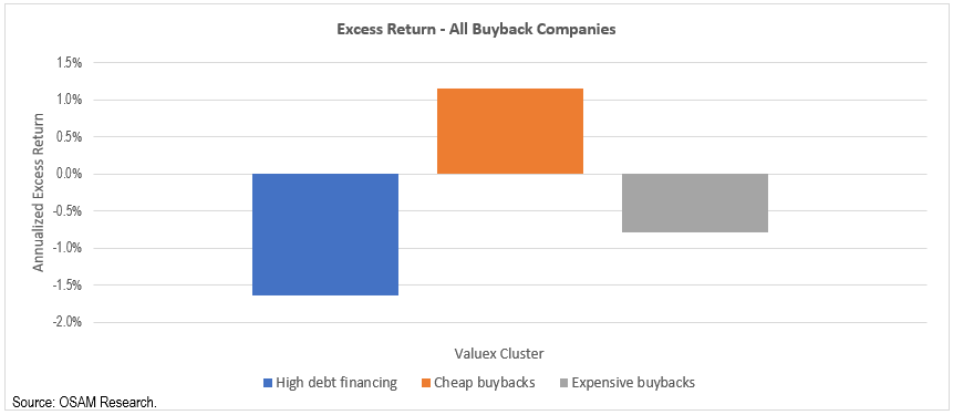
The debt financing cluster remains distinct as with our first iteration. But the two other groups stand in stark contrast measured by their current valuation:

Again, we can measure the performance of these clusters and find an interesting trend. The debt financing group confirms our earlier finding, with bad results. But the cheap buyback group outperforms the expensive buyback group by close to 2% per year, despite otherwise similar capital allocation and sourcing levels across the two groups.

Alpha Within Buybacks

When you roll this all together, you realize quickly that raw buyback yield, while powerful, can be improved with additional information (and keep in mind that for simplicity, we’ve only explored a few extra dimensions here).

To confirm, we run three traditional factor tests. We start with a universe of high buyback firms (top quintile) and then bucket those companies in quintiles based on the percent of their financing derived from operations (panel 1), the percent derived from debt issuance (panel 2), and their valuation score (panel 3). These show excess returns versus the large stocks universe. Notice the negative excess returns in the fifth quintile of the first two panels. This means that in this period, the positive effect of buybacks is undone if those companies repurchase at expensive prices or repurchase alongside the highest level of debt financing.

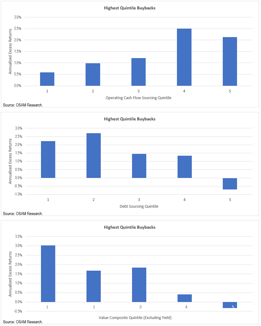
In each case, the factor returns suggest that we can improve upon a simple buyback factor.

Conclusion – The Future of Factors

One of my favorite things to do is talk to discretionary, fundamental analysts and portfolio managers. They often know their stocks and industries to a depth that is hard for a quant to fathom. When you ask them their opinion on buybacks, or valuation, or capital allocation, they inevitably respond: “it depends.” Pursuing alpha within factors is answering the question “depends on what?”

In the case of buybacks, the financing source (debt issuance vs. operating cash flows) and valuation are two of many answers. A model which adjusts for these findings represents an empirical and intuitive improvement over a simple buyback factor, which is why we use several factors measuring leverage, capital sourcing, and cash flows in our live model.

Passive and smart beta are on the rise, and fees continue to fall. Style box investing is now 25 years old. Perhaps, in the future, investors will abandon style boxes and instead focus on three simpler categories: 1) passive, 2) smart beta (commodity factors) and 3) alpha.

Nothing will work all of the time, and idiosyncratic explanations will often trump the broader observations in this letter, but our goal is always to generate alpha by tilting the odds in our clients’ favor. I believe that a process that improves upon commodity factors by finding alpha within factors gives us the best odds of doing so in the future.

We will be back with much more on this topic soon, so be sure to follow along here. Thanks to Danny Nitiutomo, CFA, a member of OSAM’s research team, for his work on this letter.

Footnotes

¹ I’m trying to avoid the phrase “machine learning” whenever possible!

² For this part of the exercise, we exclude financial firms.

ⁱ Companies can also accumulate cash, which often show up on the statement of investing cash flows in the form of marketable securities

ⁱⁱ This is not meant to be an academic paper, so I am only sharing the highlights, but for anything in production, we consider much more than these high level numbers.